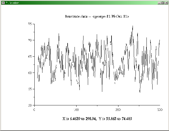
The simplest way to plot these data is to type this command into a terminal window:
plt heartrate.data
A new window will open, containing a plot as in
figure 2.2. You may be surprised to see plt exit
to the shell prompt while the window containing the plot remains
on-screen. If you run plt again, it will draw its output into
the same window as the first. This feature allows you to create
complex overlaid plots using several invocations of plt, as
described in chapter 7, beginning on
page ![[*]](crossref.png) . To dismiss the window, type an Esc (or Q, or X) into it. (If you wish to look at two or
more plots in separate windows, open a new window for plt using
xpltwin; see appendix D, beginning on
page , for details). The same capability
for creating overlays is also available when producing printed output;
see appendix B, beginning on
page , for details.
. To dismiss the window, type an Esc (or Q, or X) into it. (If you wish to look at two or
more plots in separate windows, open a new window for plt using
xpltwin; see appendix D, beginning on
page , for details). The same capability
for creating overlays is also available when producing printed output;
see appendix B, beginning on
page , for details.
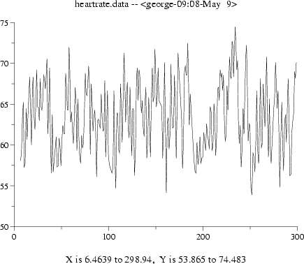
In order to illustrate the appearance of a plt screen plot, figure 2.2 was prepared from a screen dump. You can make printed plots of much better quality using plt, however, and with much less trouble than required to print a screen dump. The same plot can be printed simply by adding the optional arguments ``-T lw'' to the plt command, and then redirecting its output to lwcat, like this:
plt heartrate.data -T lw | lwcat
This command will send the plot to the default printer, producing output as in figure 2.3. Since PostScript plots are in vector rather than raster form, they can be rescaled in documents such as this without introducing artifacts, and their resolution is generally much higher than raster images despite their much smaller file sizes.
If you wish to capture the PostScript output in order to include it in a document such as this one, use lwcat's -eps option, and redirect its standard output to a file, as in:
plt heartrate.data -T lw | lwcat -eps >heartrate.eps
See appendix B for more examples and additional details about making PostScript plots and including them in other documents.