Advanced Axis Options

This chapter introduces more options for manipulating and labelling your axes, to provide fine control over the appearance of your plots.

-lx base subticks

-ly base subticks

Use these options to create logarithmic x and y axes; base is the base of the logarithms (default: 10), and subticks is either yes or no. If the axis has a small number of major ticks, plt draws subticks by default; use the subticks argument to change plt's default behavior.

The -lx and -ly options affect only how the axes are drawn; plt does not log-transform the input data, so you must provide the logarithms of the data to be plotted. Note that base does not have to be numeric; for example, ``-lx e'' will cause plt to draw a logarithmic x-axis with ticks labelled $e^0$, $e^1$, $e^2$, ... (or other integer powers of $e$ as appropriate for the range of abscissas).

-xe xmin-error xmax-error

-ye ymin-error ymax-error

These options can be used to set the amounts by which the axis ranges are allowed to exceed the ranges of the data when plt determines the axis ranges automatically.

-xm tick-base

-ym tick-base

Make axis ticks a multiple of the specified tick-base.

-xo x-axis-offset

-yo y-axis-offset

These options allow the axes to be moved from their default positions; they are particularly useful if data would otherwise be obscured by axis markings. The -xo option moves the x axis down by x-axis-offset, which is expressed as a fraction of the y axis length; the -yo option moves the y axis left by y-axis-offset, which is a fraction of the x axis length (see figure 11.4).

-xr

-yr

Use these options to plot the x axis at the top of the plot, or the y axis on the right side of the plot.

-xt x label tick-size

-yt y label tick-size

These options add an extra labelled tick at the specified $x$ or $y$ position on the corresponding axis. label can be any string; if omitted, the label is $x$ or $y$, formatted in the same way as the other labelled axis ticks. tick-size specifies the length of the tick, as a multiple of the default length for labelled ticks; if omitted, tick-size is 1. Use a negative tick-size to change the direction of the tick and the placement of the label (the result depends also on the grid-mode; see -g below).

-xts x tick-size

-yts y tick-size

Use these options to force a labelled tick to be placed at the specified $x$ or $y$ positions on the axes, and to multiply the lengths of all ticks on the corresponding axis by the factor tick-size (other than any extra ticks generated using -xt or -yt). Use a negative tick-size to change the direction of the tick and the placement of the labels (the result depends also on the grid-mode; see -g below).

-g grid-mode ...

The -g option accepts one or more grid-mode specifiers, which define how to create a grid. Note that if more than one grid-mode is supplied, they must be surrounded by quotes or separated by commas, because -g takes only one string as its argument. The defined grid-modes are:

in	puts ticks inside the grid
out	puts ticks outside the grid (default)
both	puts ticks inside and outside the grid
none	suppresses ticks
sym	make symmetric axes (at top and right)
grid	make a full grid (extend major ticks across the entire plot)
xgrid	extend major x axis ticks across the entire plot
ygrid	extend major y axis ticks across the entire plot
sub	make a fine grid (extend all ticks across the entire plot)

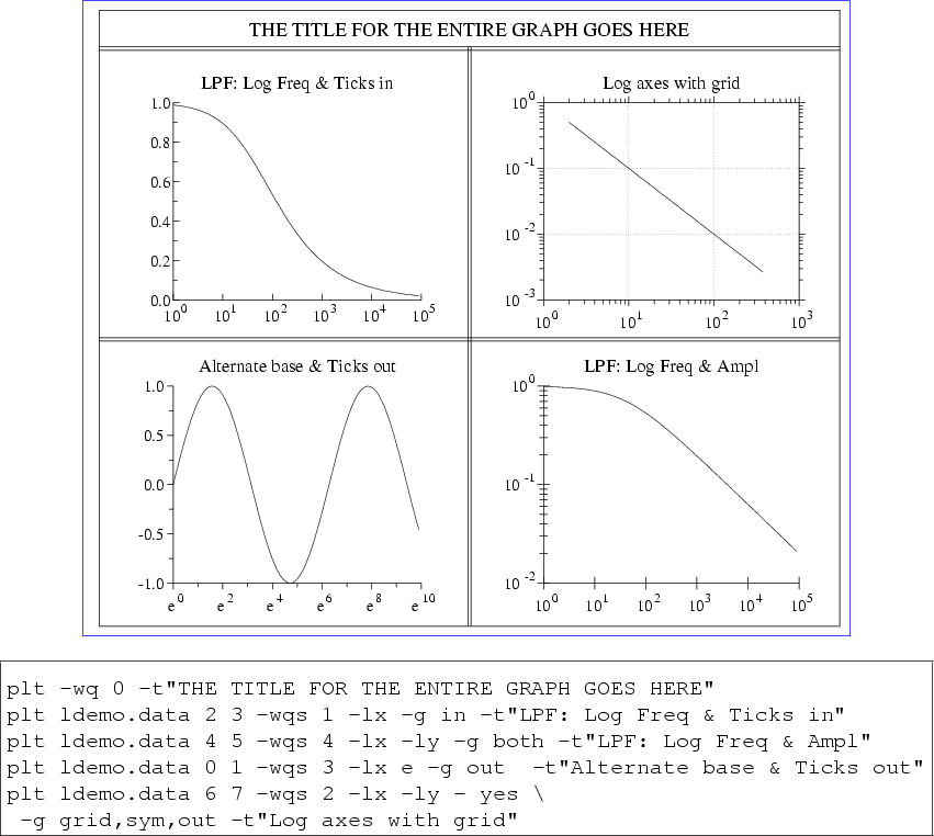
Figure 12.1 demonstrates several of these options, featuring logarithmic axes and a variety of grid modes. The data file, ldemo.data, is included in the doc directory of the plt distribution (see appendix F).

Figure 12.1: This example demonstrates several of the advanced axis options. It was produced using these commands:

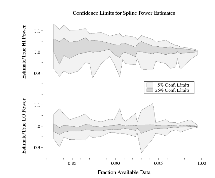
As a final example, figure 12.2 demonstrates use of the O plotstyle, the -yo option for shifting the y axis to the left, the -xts option to create an extra labelled tick mark, the -size option (see appendix B), relative parameter values in transient fontgroup specifications, overlays, and multiple plot windows. The figure was created using the following commands:

plt power.data 0 1 2 3 4 5 -F"
size .7 5 5
sf p W1
W - .1 - .47
# P*1.5 means multiply point size by 1.5.  The point size for the 'O'
# plot type has no effect on the plot, but changes the height of the
# box in the legend.
p 0,1,5O(G.95,P*1.5) 0,2,4O(G.85)
lp .7 1.2 .9
le 0 0   5% Conf. Limits
le 1 1 25% Conf. Limits
t
y Power Error
yo 0.02
y Estimate/True LO Power
xts .85
xa .82 1 .01 - 5
x Fraction Available Data"

plt power.data 0 6 7 8 9 10 -F"
s ex
size .7 5 5
sf p W1
W - .53 - .9
p 0,1,5O(G.95,P*1.5) 0,2,4O(G.85)
t Confidence Limits for Spline Power Estimates
xts .85
xa .82 1 .01 - 5
y Estimate/True HI Power
yo 0.02"

The data file, power.data, is included in the doc directory of the plt distribution (see appendix F).

Figure 12.2: A complex plot (see text).